Demo of the LAMINAR package
[1]:
import LAMINAR

import torch
import numpy as np
import matplotlib.pyplot as plt

from sklearn.datasets import make_moons
from LAMINAR.utils.tensor_visualisation import get_cov_colours
[2]:
# make moon dataset and fix two specific points for distance tests

d = np.array([[1.25, -2.0], [-0.65, 1.0]])  # special points

X, Y = make_moons(n_samples=1498 *2, noise=0.1) # moon dataset
X = X[Y == 0] # upper moon
X = (X - X.mean(axis=0)) / X.std(axis=0)    # standardise

X = np.append(d, X, axis=0) # combine

# make a tensor
data = torch.tensor(X, dtype=torch.float32) # to torch tensor
data.shape
[2]:
torch.Size([1500, 2])
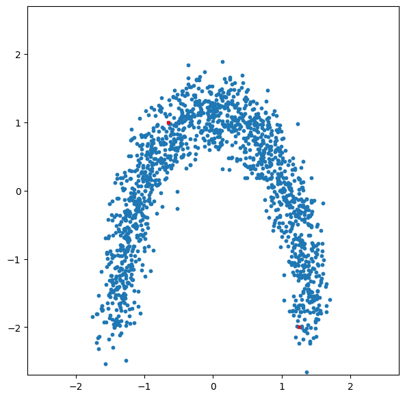
[3]:
# visualize the dataset
plt.figure(figsize=(7, 7))
plt.ylim(-2.7, 2.7)
plt.xlim(-2.7, 2.7)


plt.scatter(X[:, 0], X[:, 1], s=10);
plt.scatter(X[0, 0], X[0, 1], s=10, marker='x', c='r');
plt.scatter(X[1, 0], X[1, 1], s=10, marker='x', c='r');
[11]:
# initialize the LAM class and train
LAM = LAMINAR.LAMINAR(data, epochs=500, save_distance_matrix=False)
Iteration 0 | Train Loss: 1056.7645833333333 | Validation Loss: 564.425048828125
Iteration 99 | Train Loss: 207.44392740885417 | Validation Loss: 223.6324462890625
Iteration 199 | Train Loss: 188.49836975097656 | Validation Loss: 187.03955078125
Iteration 299 | Train Loss: 187.07679341634116 | Validation Loss: 196.35438537597656
Iteration 399 | Train Loss: 182.43506388346353 | Validation Loss: 186.2667694091797
Iteration 499 | Train Loss: 184.21164082845053 | Validation Loss: 185.3126220703125
[12]:
# plot loss hist and check for convergence
plt.plot(LAM.loss_hist['train'], linewidth=0, marker='.')
plt.plot(LAM.loss_hist['val'], linewidth=0, marker='.')
plt.yscale('log')
plt.xlabel('Epoch x100')
[12]:
Text(0.5, 0, 'Epoch x100')

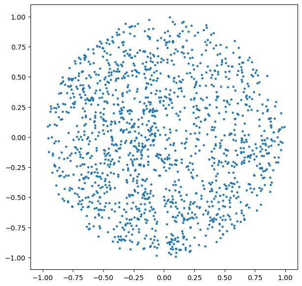
[13]:
# visualize the pushed data and check for uniformness
plt.figure(figsize=(7, 7))
plt.ylim(-1.1, 1.1)
plt.xlim(-1.1, 1.1)
plt.scatter(LAM.X_pushed[:, 0], LAM.X_pushed[:, 1], s=5);
[14]:
# function for visualisation

def vis(data, tensors, xlim, ylim):
    col = get_cov_colours(data, tensors)

    plt.figure(figsize=(7, 7))
    plt.xlim(-xlim, xlim)
    plt.ylim(-ylim, ylim)

    # make everythin numpy
    col = np.array(col)

    #col = np.ones((data.shape[0], 4))

    # for each data point, claculate the eccentricty of the respective tensor,a s well as the angle
    for i in range(data.shape[0]):
        eigenvalues, eigenvectors = np.linalg.eig(tensors[i])
        eig_idx = np.argmax(eigenvalues)
        vec = eigenvectors[:, eig_idx]

        angle = np.arctan2(vec[1], vec[0])
        angle = np.degrees(angle)

        if angle < 0:
            angle += 360

        angle += 90

        b = tensors[i][0][1]
        c = tensors[i][1][1]
        a = tensors[i][0][0]

        e = np.sqrt((2*np.sqrt((a-c)**2 + 4*b**2))/((a+c) + np.sqrt((a-c)**2 + 4*b**2)))

        e = e**10 * 2

        # at location data[i], plot a an arraow, pointing in both directions at the angle
        plt.arrow(data[i, 0], data[i, 1], 0.05* e * np.cos(np.radians(angle)), 0.05* e * np.sin(np.radians(angle)),
                  head_width=0.05, head_length=0.05, fc=col[i], ec='k', alpha=1, width=0.02, linewidth=0.5)
        plt.arrow(data[i, 0], data[i, 1], -0.05* e * np.cos(np.radians(angle)), -0.05* e * np.sin(np.radians(angle)),
                  head_width=0.05, head_length=0.05, fc=col[i], ec='k', alpha=1, width=0.02, linewidth=0.5);
[15]:
tensors = LAM.net.metric_tensor(data)

vis(data, tensors, 2.7, 2.7)

[16]:
# rference for colours

from LAMINAR.utils.tensor_visualisation import plot_reference
plot_reference()

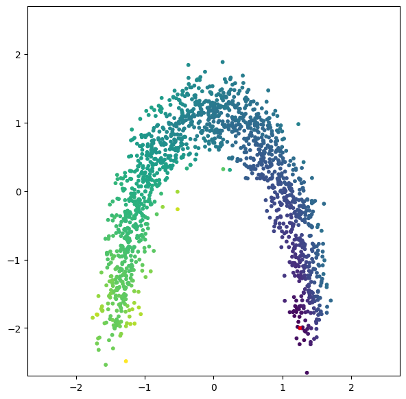
[17]:
# get distances of points to data[0] and show
idx, dists = LAM.query(data[0])

plt.figure(figsize=(7, 7))
plt.ylim(-2.7, 2.7)
plt.xlim(-2.7, 2.7)
# plot the points with dists as colour
plt.scatter(data[idx, 0], data[idx, 1], s=10, c=dists, cmap='viridis')

# plot original point in red with marker X
plt.scatter(data[0, 0], data[0, 1], s=10, c='r', marker='x');
[18]:
# also plot euclidean distance for comparison
euclidean_dists = torch.norm(data[0] - data[:], dim=1)

print(euclidean_dists.shape)

plt.figure(figsize=(7, 7))
plt.ylim(-2.7, 2.7)
plt.xlim(-2.7, 2.7)
plt.scatter(data[:, 0], data[:, 1], s=10, c=euclidean_dists)
plt.scatter(data[0, 0], data[0, 1], s=10, c='r', marker='x');
torch.Size([1500])

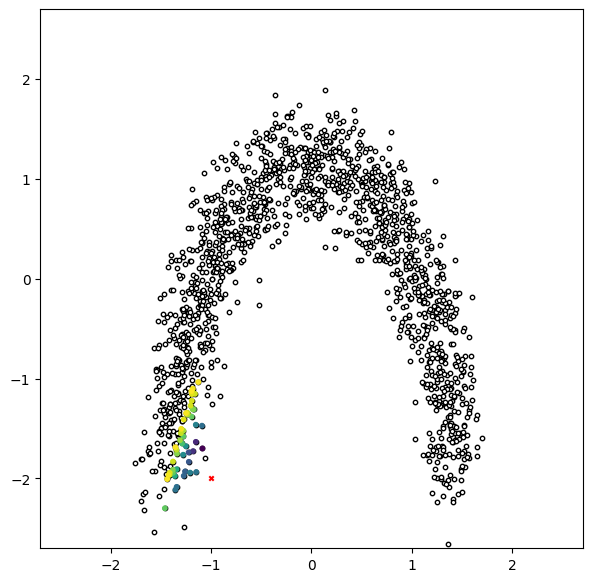
[19]:
# get closest points to the arbitrary point (-1, -2)
idx, dists = LAM.query(torch.tensor([-1, -2], dtype=torch.float32), 50)

plt.figure(figsize=(7, 7))
plt.ylim(-2.7, 2.7)
plt.xlim(-2.7, 2.7)

# plot all data points in white with black edges
plt.scatter(data[:, 0], data[:, 1], s=10, c='w', edgecolor='k')

# plot the closest points wth dists as colour
plt.scatter(data[idx[0, 1:], 0], data[idx[0, 1:], 1], s=10, c=dists[0, 1:], cmap='viridis')

# plot original point in red with marker X
plt.scatter(-1, -2, s=10, c='r', marker='x');
[20]:
# get closest points for first three datapointsand their distances
idx, dists = LAM.query(data[:3], 5)

print(idx)
print(dists)
tensor([[   0, 1368,  982,  166,  910],
        [   1, 1013, 1279,  454,   60],
        [   2,  312,  796,  986,  283]])
tensor([[0.0000, 0.0450, 0.0634, 0.1042, 0.1189],
        [0.0000, 0.0284, 0.0490, 0.0652, 0.0858],
        [0.0000, 0.0132, 0.0287, 0.0288, 0.0451]])
[21]:
# full distances and points in order for point 0
LAM.query(data[0])
[21]:
(tensor([[   0, 1368,  982,  ...,  105,  280, 1115]]),
 tensor([[0.0000, 0.0450, 0.0634,  ..., 5.1347, 5.2534, 5.7081]]))
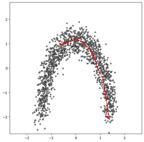
[22]:
# get approximate ditance between first two points
dist, path = LAM.distance_approx(data[0], data[1], return_path=True)

print(dist)

# plot the path on the data
plt.figure(figsize=(7, 7))
plt.ylim(-2.7, 2.7)
plt.xlim(-2.7, 2.7)

plt.scatter(data[:, 0], data[:, 1], s=10, c='w', edgecolor='k')
plt.plot(path[:, 0], path[:, 1], c='r', linewidth=1)
plt.scatter(path[:, 0], path[:, 1], s=10, c='r')
plt.scatter(data[0, 0], data[0, 1], s=10, c='r', marker='x')
plt.scatter(data[1, 0], data[1, 1], s=10, c='r', marker='x');
[2.6861117]
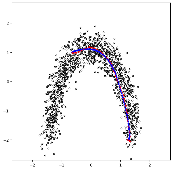
[23]:
# smoothen path
dist, action, path_smooth = LAM.distance_smooth(start=data[0], end=data[1], n=100, num_hidden=256, num_layers=5)
Final loss: 0.0014995024539530277
Learning rate reduced to 1.0000000000000002e-06
Learning rate reduced to 1.0000000000000002e-07
Learning rate reduced to 1.0000000000000004e-08
Learning rate reduced to 1.0000000000000005e-09
Best loss: 4.264859676361084
Final loss: 4.264859676361084
[24]:
# plot the path on the data
plt.figure(figsize=(7, 7))
plt.ylim(-2.7, 2.7)
plt.xlim(-2.7, 2.7)

plt.scatter(data[:, 0], data[:, 1], s=10, c='w', edgecolor='k')

plt.plot(path[:, 0], path[:, 1], c='r', linewidth=1)
plt.scatter(path[:, 0], path[:, 1], s=10, c='r')


plt.plot(path_smooth[:, 0], path_smooth[:, 1], c='b', linewidth=1)
plt.scatter(path_smooth[:, 0], path_smooth[:, 1], s=10, c='b')


plt.scatter(data[0, 0], data[0, 1], s=10, c='r', marker='x')
plt.scatter(data[1, 0], data[1, 1], s=10, c='r', marker='x')

print('Length: ', dist)
print('Action: ', action)
Length:  tensor([2.7795])
Action:  tensor(4.2649)
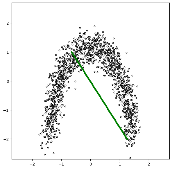
[25]:
#euclidean interpolation for comparison

eucl_path = torch.linspace(0, 1, steps=100)
eucl_path = data[0] + (data[1] - data[0]) * eucl_path[:, None]

plt.figure(figsize=(7, 7))
plt.xlim(-2.7, 2.7)
plt.ylim(-2.7, 2.7)

plt.scatter(data[:, 0], data[:, 1], s=10, c='w', edgecolor='k')
plt.scatter(eucl_path[:, 0], eucl_path[:, 1], s=10, c='g')
[25]:
<matplotlib.collections.PathCollection at 0x22bde1559d0>